



Key takeaways of the article
- In a tropical or monsoon climate, a convective cell is born, peaks and is gone inside the hour, and a plant underneath it can lose half its output in minutes.
- Satellite imagery and numerical weather prediction lose their grip below the hour: a revisit of ten to fifteen minutes and a pixel of a few kilometres cannot resolve a cell of a few kilometres that lives for twenty minutes.
- Over ninety-six days on an operating tropical plant, a learning model using on-site data cuts error by 25% against numerical weather prediction and 24% against persistence at two hours, while below twenty-one minutes persistence still wins.
- A ground-based network of hemispherical cameras fills that window, adding an average of 20% of skill below thirty minutes on a site that already has pyranometers.
In a tropical or monsoon climate, a convective cell is born, peaks and is gone inside the hour, over a few square kilometres. Under it, a photovoltaic plant can lose half its output in minutes and recover just as fast. That is not a modelling curiosity. It is the timescale on which an operator commits energy to the market, decides whether to charge or hold a battery, and pays for the difference between what was declared and what was delivered.
This article sets out the work presented at The smarter E South America in Sao Paulo in August 2026: where satellite imagery and numerical weather prediction stop carrying information in a tropical climate, what ninety-six days of measured data on an operating plant show, and what a network of ground-based cameras puts in their place.
What has changed on the Brazilian grid
Curtailment, storage, and a plant that is dispatched
The transmission network no longer carries everything the plants generate at midday. Output exceeds what the lines can move south, and the surplus is curtailed. At the same time, battery storage is being installed alongside the arrays, which turns a passive asset into a controlled one: charge, hold or deliver becomes a decision, and that decision is revised every few minutes.
Solar-powered hydrogen projects add a third layer, because an electrolyser has to be scheduled against the irradiance it will actually receive, not against a daily average.
The price signal has inverted
Put the Nordeste settlement price against measured production over May to August 2026 and the pattern is plain: the hours of highest output are no longer the hours of highest value. Production peaks in the middle of the day, when the price collapses below the PPA reference, and the price recovers in the late afternoon, exactly as the plant fades.
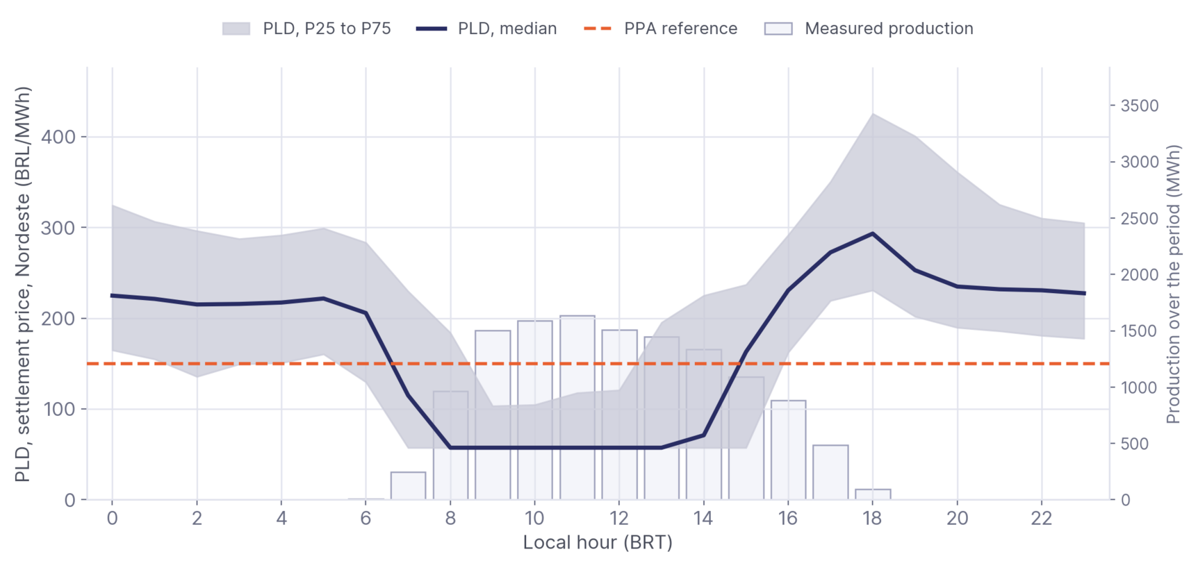
An operator now needs two distinct things from the same plant: short-term forecasting, to decide what to dispatch and what to bid, and measurement, to know what the plant actually did.
Convective cells are not fronts, and that is the whole problem
Why extrapolation works in temperate latitudes
Almost every operational forecasting method in use today was designed against mid-latitude weather. There, cloud fields are organised by synoptic fronts. The structures are large, vertical convection is limited, and advection is driven by upper-level flow that stays coherent for hours. A cloud observed now is, to a useful approximation, the same cloud somewhere else later. Extrapolation works because there is something to extrapolate.
Why it does not transfer
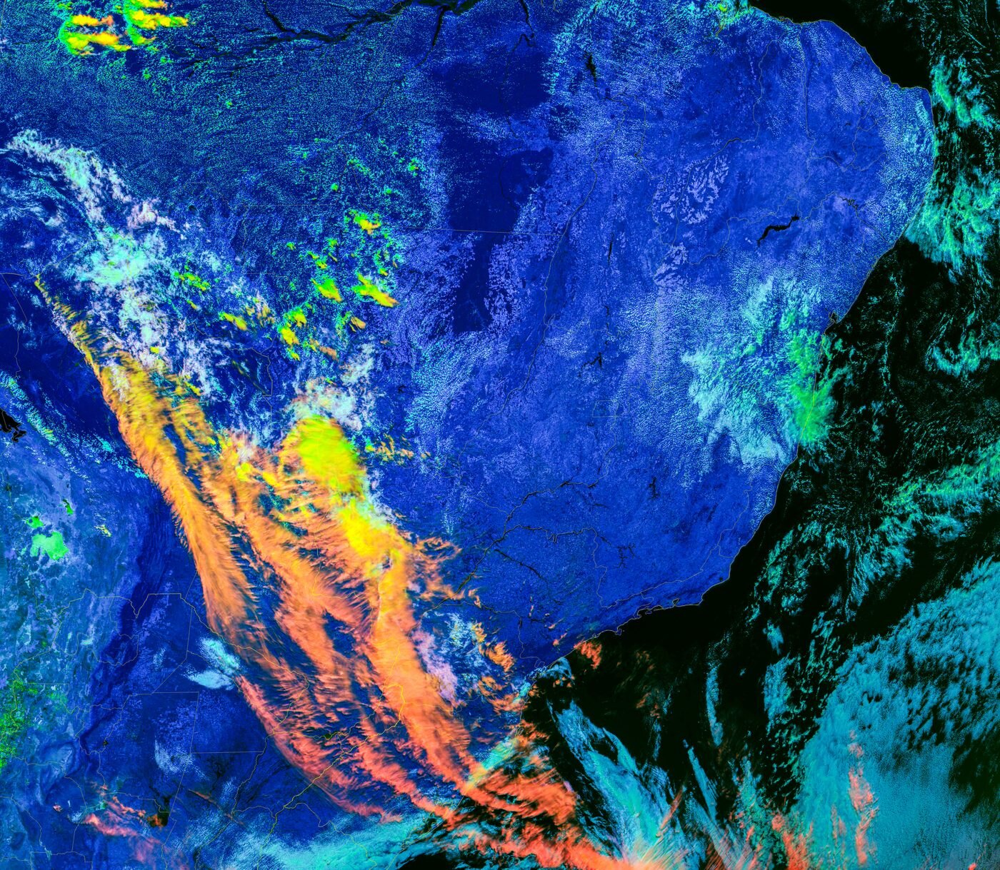
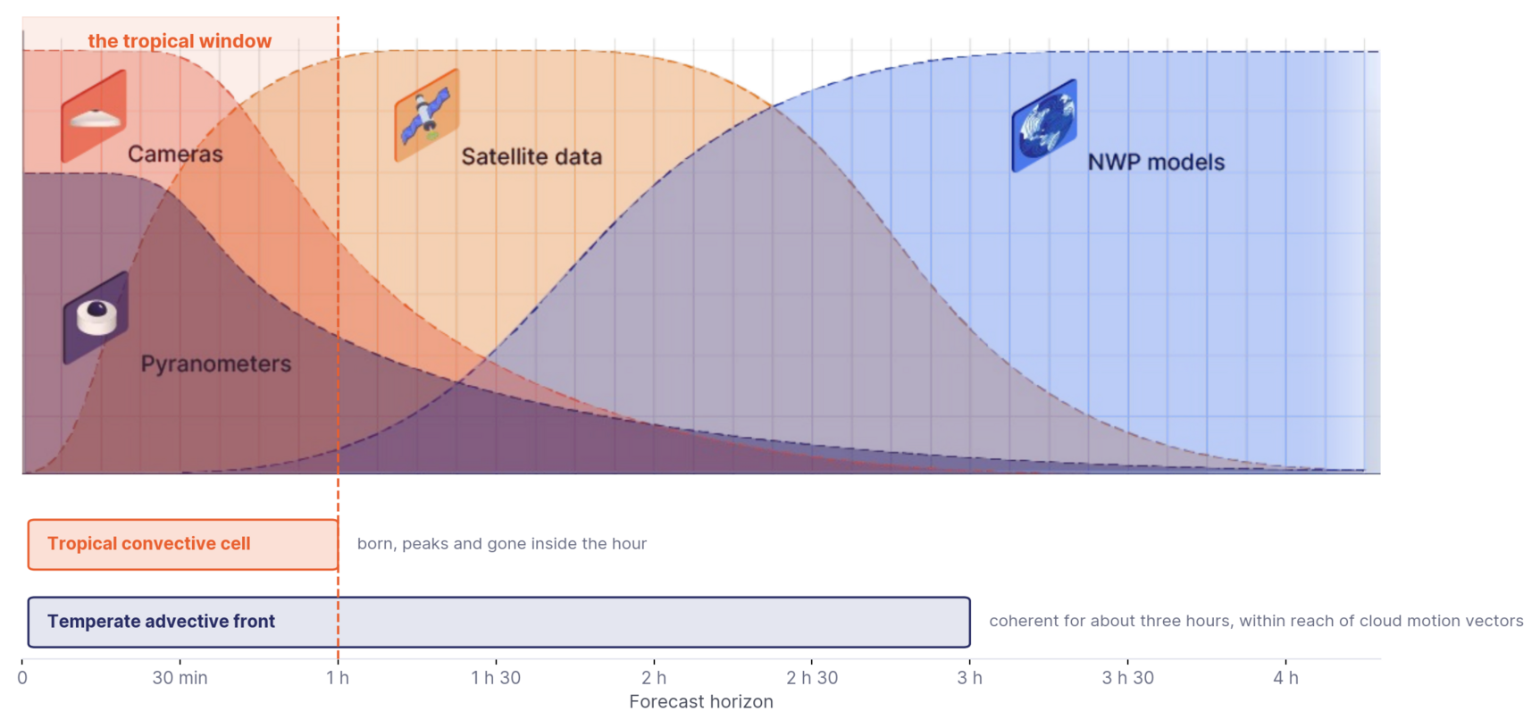
Continental tropical latitudes behave differently. Cells form by surface heating over a few square kilometres, develop vertically rather than travelling, and dissipate close to where they appeared. There is little coherent advection, and coherent advection is precisely what cloud motion methods rely on. The methods are not being applied badly in Brazil. They are being applied to a phenomenon they were not built for.
What the satellite sees, and what the ground measures
Two days, two instruments
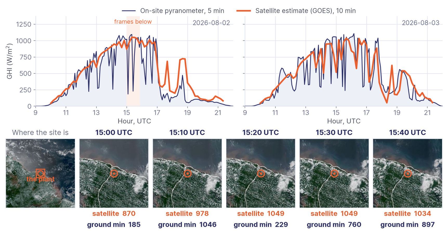
The gap is easiest to see on a single site. Take two days of global horizontal irradiance on an operating plant in French Guiana, a climate recognised as one of the most variable in the world when averaged over a full year, with a satellite product derived from GOES at ten minute resolution, and put it against a pyranometer on the same site sampling every five minutes.
The two curves agree on the shape of the day and disagree on everything that matters inside the hour. The satellite estimate is smooth. The ground measurement is a comb: drops of several hundred watts per square metre, lasting a few minutes, entirely absent from the satellite record.
Under each satellite frame in the strip below, the figure gives the satellite estimate and the lowest irradiance actually measured in the ten minutes that followed. At 15:20 UTC the satellite reads 1049 watts per square metre. The ground fell to 229 in the interval that followed. At 15:00, satellite 870 against a ground minimum of 185. The plant has already been through a ramp that neither the pixel size nor the refresh interval could resolve.
A mismatch of scale, and a latency nobody counts
This is not a defect of the satellite product. It is a mismatch of scale and timing: a revisit of ten to fifteen minutes and a pixel of a few kilometres cannot resolve a cell of a few kilometres that lives for twenty minutes.
And the comparison above is generous to the satellite, because it uses the nominal timestamp of the image. The processing and delivery latency between acquisition and the moment the estimate reaches an operator is not counted in it. In operation, the gap is wider than the figure shows.
Where each source actually carries information
Read that way, the question stops being which product is best and becomes which source carries information at which horizon.
Numerical weather prediction owns the day-ahead and the hours ahead. Satellite imagery owns the range between roughly one hour and two and a half hours, where cloud fields still hold together. Below the hour, in a convective climate, both fade, and what remains is what can be measured and seen from the ground: pyranometers for the state of the plant now, cameras for what is about to arrive.
Ninety-six days, three methods, one plant
The protocol
To size the effect rather than argue about it, we ran a continuous evaluation on an operating tropical site from 1 May to 4 August 2026, ninety-six days without selection. A forecast was issued every fifteen minutes and compared with the output the plant actually delivered. Three methods ran on identical data.
Persistence. Assume the sky stays as it is now. It requires a sensor and nothing else, and in a convective climate it is a serious competitor at very short horizons.
Numerical weather prediction alone. A model on a grid of several kilometres, refreshed a few times a day.
A learning model using on-site data, combined with satellite imagery and NWP inputs.
Three numbers come out of the record
Error is given as a percentage of mean output, so the figures transfer to a plant of any size. Restricted to the horizons that matter for dispatch, under two hours, the record gives 25% of skill against numerical weather prediction at two hours, 24% against persistence at the same horizon, and a crossing point at 21 minutes, below which persistence still has the lowest mean absolute error of the three.
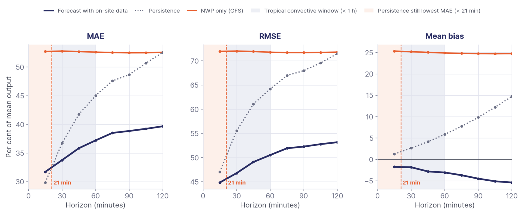
That last number is the interesting one, because it says exactly where the remaining problem lives. Between zero and twenty-one minutes, none of the large-scale data sources carries information, and the best available answer is to assume nothing changes. Something else has to fill that window.
What an operator actually experiences
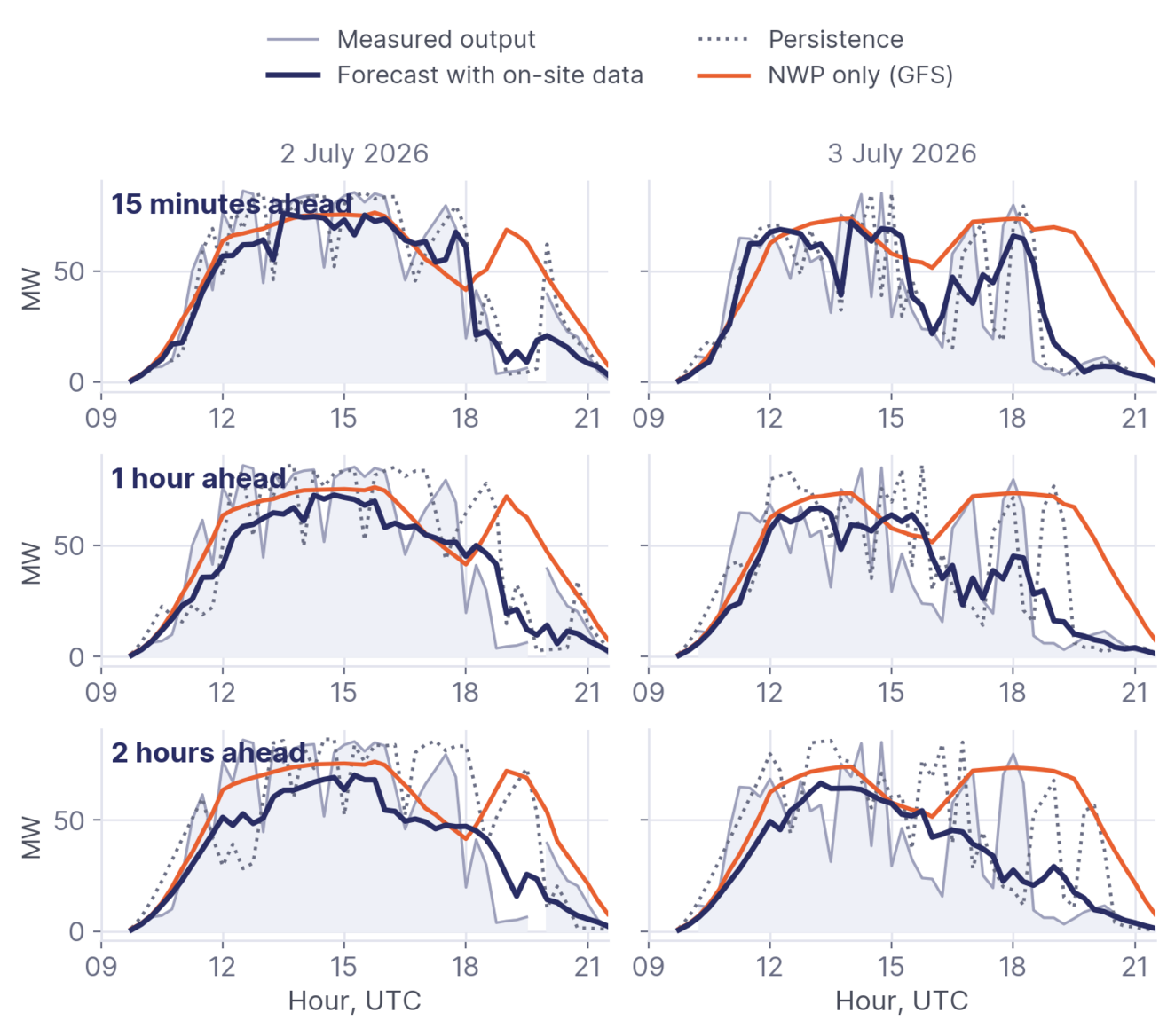
Aggregate error hides what happens on a given afternoon. Two days of the record, at three horizons, show it directly. Persistence tracks the plant with a lag of one step, which is worthless the moment a ramp starts. The weather model holds a plausible plateau and misses the late afternoon collapse entirely. The model using on-site data follows the envelope of the day, including the collapse, at all three horizons.
Below thirty minutes, only the sky itself
Four processing steps, run on site
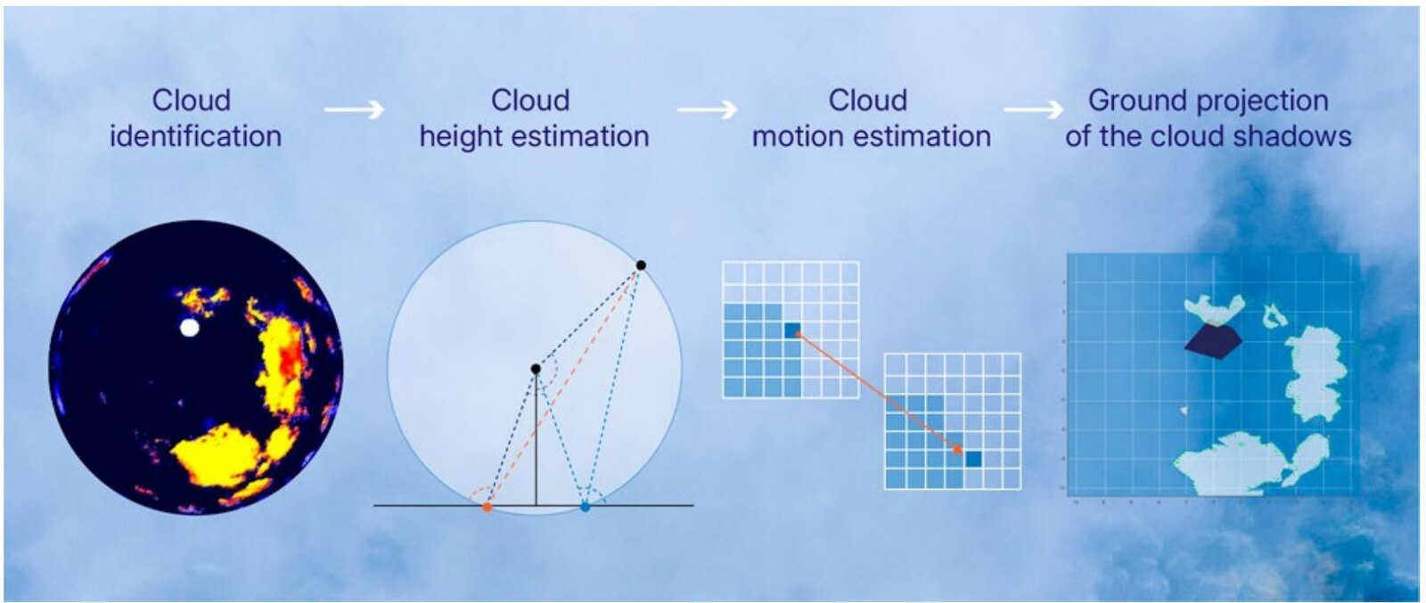
The instrument that fills the window is the sky above the plant, observed from the ground. A network of hemispherical cameras watches the approaching cloud field. Several imagers observing the same sky from different points allow a cloud to be located in three dimensions rather than merely seen, and its shadow to be projected onto the plant layout.
Four steps run continuously on site: identify the clouds in the hemispherical image, estimate their height, estimate their motion, then project the shadows onto the ground. The output is the next thirty minutes of expected output for the plant, refreshed continuously.
Twenty per cent, on top of ground measurement
On a site already equipped with pyranometers, the camera network adds an average of 20% of skill below thirty minutes. That gain is not measured against a naive baseline. It is measured on top of an installation that already has ground measurement, which is the only comparison an operator should accept.
The same instruments serve twice
There is a practical argument that often decides the question, and it has nothing to do with forecasting. The instruments installed for forecasting are the same ones that answer the operational questions.
Before construction, a reference station calibrates the satellite record, which carries a bias in tropical climates, and characterises the ramps a battery would have to absorb. Once the plant is running, a pyranometer network makes curtailment and soiling losses separable and quantified, and resolves variability at the timescale the plant actually experiences rather than at the timescale of a monthly report.
One instrumentation, two uses. That is usually what makes the business case close.
What this means for an operator
If your plants sit in a convective climate and your dispatch decisions are taken inside the hour, three statements follow from the measured record.
The horizon that matters to you is the one where satellite imagery and weather models are weakest, and no amount of post-processing moves that boundary. On-site measurement is not an accessory to the forecast below the hour, it is the dominant source of information. And the same sensors pay for themselves twice, once in forecast accuracy and once in knowing what the plant did.