




Key takeaways of the article
- Global NWP models solve partial differential equations across 131+ million grid points, with forecast cycles refreshed every six hours at synoptic times, the backbone of all operational weather forecasting.
- Supercomputing power of up to 29 petaflops is required to process weather data and produce real-time, accurate forecasts at national and global scale.
- The chaotic nature of the Earth's atmosphere means that even minor errors in initial conditions amplify rapidly over time, making data collection and data assimilation critical to forecast skill.
- Ensemble forecasting runs multiple simulations with perturbed initial conditions to quantify uncertainty and support decision-making around severe weather events, tropical cyclones, and high-impact weather phenomena.
What are numerical weather prediction (NWP) models?
The weather forecasts we access daily, on television, through dedicated software, or on mobile platforms – are produced by numerical weather prediction models, commonly referred to as NWP models. These mathematical models simulate the evolution of weather systems by solving sets of physical equations over a discrete computational grid, producing the computer-generated predictions that forecasters and automated services rely on.
Definition: A Numerical Weather Prediction (NWP) model simulates the future state of the atmosphere by numerically solving equations governing fluid dynamics, thermodynamics, and radiation across a three-dimensional grid of points.
These primitive equations, a form of partial differential equations derived from fundamental physics, govern the rates of change in temperature, wind, water vapor, and precipitation across the full atmospheric column. They form the mathematical core from which all modern weather forecast models are built.
The major meteorological centers behind NWP forecasts
Extraordinary demands on computing infrastructure
Atmospheric modeling at global scale places extreme demands on computational resources and storage capacity. Producing real-time forecasts across national or global regions requires supercomputing infrastructure that only a handful of organizations worldwide can support. As a result, global medium-range weather forecasts are produced by a small number of major national and international meteorological centers.
Among the most well-known are:
- ECMWF, the European Centre for Medium-Range Weather Forecasts
- NOAA, the National Oceanic and Atmospheric Administration (United States)
The supercomputers operated by these organizations frequently rank among the most powerful in the world at the time of their commissioning. For instance, Météo-France’s supercomputer was ranked 30th globally when installed in 2020.
These centers produce global forecasts with a spatial resolution typically ranging from 10 to 50 km, depending on the model.
Forecast cycles: Updates every six hours
To limit the divergence of simulations over time, forecasts are regularly refreshed. Global NWP models are rerun every six hours at the synoptic hours, 00:00, 06:00, 12:00, and 18:00 UTC – ensuring that current weather observations are continuously integrated into the forecast process. These successive updates constitute the forecast cycles.
29 Petaflops: The scale of computational power required
NOAA’s supercomputer operates at approximately 29 petaflops, that is, 29 × 10¹⁵ mathematical operations per second. This level of processing power is required to solve the complete set of atmospheric equations across hundreds of millions of grid points within operational time constraints. It explains why only a small number of major centers worldwide are capable of producing global-scale weather forecasts autonomously.
Inside a numerical weather prediction model: Grid, resolution, and data points
How the atmosphere is discretized
A numerical weather prediction model is based on solving a set of mathematical equations over a computational grid. The Earth’s surface is discretized along latitude and longitude, and also vertically by altitude, this is referred to as the spatial resolution of the model.
The GFS model:A concrete example
Consider NOAA’s Global Forecast System (GFS). Its horizontal resolution is approximately 28 km (0.25°). This means that meteorological variables, such as wind speed or temperature, are computed at regular intervals of roughly 25 to 30 km, representing approximately 1,440 × 720 grid points at the surface, or more than one million points in total.
These surface points are then extended vertically to represent the structure of the atmosphere at altitude. The GFS model comprises 127 vertical levels, resulting in more than 131 million computational grid points.
Parameter
GFS Value
Horizontal resolution
~28 km (0.25°)
Surface grid (lat × lon)
1,440 × 720
Vertical levels
127
Total grid points
> 131 million
Time step
7 min 30 sec
Forecast horizon
Up to 15 days
Time steps per run
2,880
Meteorological variables
> 150
Supercomputer power (NOAA)
~29 petaflops

The temporal dimension
To this spatial dimension is added the temporal dimension. To represent the evolution of the atmosphere, the model computes the state of these millions of points at regular time intervals. In the case of GFS, calculations are performed every 7 minutes and 30 seconds, over a forecast horizon of up to 15 days, corresponding to 2,880 time steps.
Taking into account that the model produces more than 150 meteorological variables, each requiring numerous mathematical operations, the critical importance of both substantial computational power and adequate storage capacity becomes self-evident.
Uncertainties and errors in NWP Models
Approximating a continuous atmosphere
Numerical models provide forecasts on discrete spatial and temporal grids. They therefore constitute an approximation of atmospheric phenomena that are, by nature, continuous. The numerical methods used to solve the physical equations also introduce uncertainties.
Furthermore, the model’s initial state, the description of the atmosphere at the start of the forecast, inevitably contains errors, which tend to amplify over time.
Improving accuracy: Resolution and physical parameterization
Reducing these errors may be achieved by increasing the spatial and temporal resolution, but this entails significantly higher computational costs as well as an adaptation of the physical parameterizations to represent smaller-scale phenomena. Improving these physical schemes has been an active area of research for several decades.
Data assimilation: Combining models with real-world observations
To mitigate errors in the initial state, data assimilation methods play a central role. These consist in optimally combining the model’s physical equations with all available observations:
- Surface measurements
- Satellite observations
- Airborne data
- Radiosonde profiles
These methods make use of observations gathered in the hours preceding the model run and require multiple successive simulations. They therefore demand both a large volume of data and considerable computational power to produce an initial state as close as possible to observed reality.
Applications: From global forecasts to regional models
Who can access NWP outputs?
Only major national or international meteorological centers possess the necessary resources, computational power, storage capacity, and international cooperation for data sharing, to carry out all of these operations. Their forecasts are, for the most part, publicly accessible.
Global forecasts as boundary conditions for regional models
These global forecasts can be used directly, but can also serve as boundary conditions for higher-resolution regional models. The latter enable the study of local phenomena or the production of specific applications, such as wind or solar resource atlases.
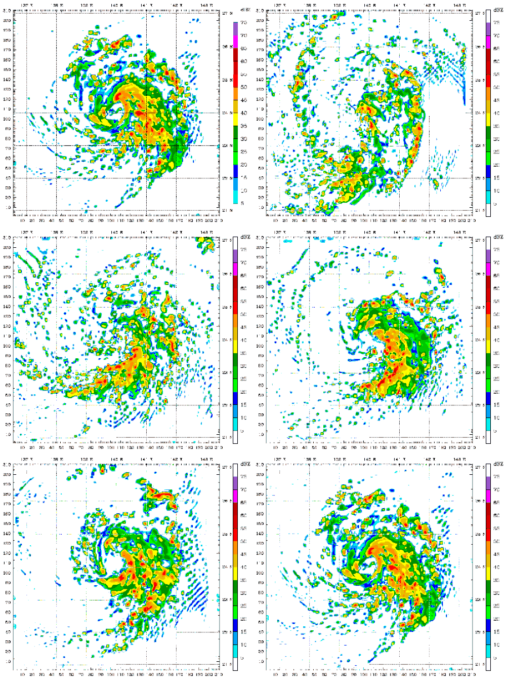
The most widely used public model in this context is the Weather Research and Forecasting (WRF) model.
Conclusion
Numerical weather prediction models are complex mathematical tools that simulate the evolution of the atmosphere over a discrete spatio-temporal domain based on physical equations. Their accuracy continues to improve, at the cost of ever-increasing computational demands. Forecast cycles ensure the regular updating of simulations, while the data produced can be exploited at both global and local scales through limited-area models.